Computing power in abundance? - Intelligence versus pure power

An appeal to the computational engineers to use more brains again
Again and again, I encounter calculation models with my employees and also with our customers that are insanely complicated and unfortunately take so long to calculate that no reasonable optimizations can be made in a timely manner. The end results are dissatisfied customers who receive the necessary results for their conclusions too late.
Since I had very limited resources in my early days as a computational engineer in the late 1980s, I depended on solving problems intelligently rather than with power (computational power).
Computational power has increased by more than a factor of 1,000,000 in my company alone in the 32 years I have now been in business.
But now
Power = work per time spent
If you only use the increased computing power and at the same time think less and less about how to intelligently reduce the required computing time, you waste resources and the performance is worse than it could be.
This is comparable to a car with a holey tank, where more and more powerful engines are installed to save fuel.
Basics
Let's look at the basics.
Numerics, whether flow simulation or structural simulation, is fundamentally about discretizing.
Discretizing means selecting finitely many (discrete) points from a large number of possible points (the continuum) at which you want results.
Why? Even the most powerful computer has its problems with infinity.
The most general case for a simulation means that the results change with time in space.
So you also have to discretize the time to be able to determine the temporal behavior.
If in reality a value changes strongly (spatially or temporally), the density of discrete points must be larger than in areas where the results remain almost constant. Otherwise, nothing useful will come out of it.
An example of this is the stresses in a notch radius. One element over the radius is simply not enough.
Also the distances between the points should not increase or decrease abruptly, because then the solution algorithms get difficulties.
Computing time
The required computing time is approximately quadratic to the number of points (nodes, elements, volumes, particles) and linear to the time steps.
Therefore, intelligent model building / meshing should start with the number of elements first.
The spatial discretization
The number of elements can be drastically reduced by using symmetry properties. However, suitable boundary conditions have to be chosen at the symmetry planes, which is not always easy and where mistakes are often made.
Thin structures can be described much more accurately using shell elements and calculate faster. Bar-like structures can be calculated much more efficiently by using beams.
And there is the plane stress state, the plane strain state and the rotationally symmetric state, which could also be used. Very few people still know the difference between plane stress state and plane strain state.
Simplifications in the model
In the flow domain, for example, perforated plates can be simplified by porous media and a model with several million
volume elements becomes a model with 500,000 elements. Calculation times can thus quickly be reduced by a factor of 10 - 100.
Another tip: If the thickness of the porous medium is increased and the porosity is reduced, the convergence behavior improves considerably. The results are hardly influenced by this.
Example:
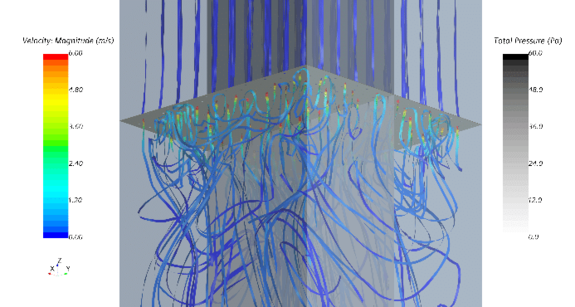
The determination of the pressure drop through a 1 m x 1 m perforated screen can be described by.
- A 3D simulation of the entire model (Figure 1)
- A 3D simulation of a section
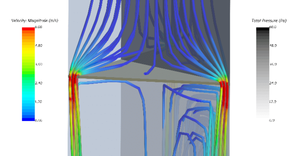
- A 3D simulation of a symmetrical model of a hole with corresponding boundary conditions (Figure 2).
The result: almost identical, the deviation is < 3%. Computation times drop from 1 hour to less than 1 minute. This is almost two orders of magnitude!
If one now calibrates a porous medium, the perforated plate in the overall model can thereby be replaced and global statements can be made in the range of minutes instead of waiting days.
The time discretization
Often the time step size is kept constant in calculations, although the results behave logarithmically. A logarithmic time step size dramatically reduces computation time and memory requirements.
Logarithmic behavior is the case, for example, with creep, temperature trends, or concentration trends.
Try to use an adjusted time scale instead of constant time steps. To avoid odd time points, I used the following time steps here:
1,2,5,10,20,50,100,200,500,1000,2000,5000,10000 ….
200,000 hours of creep (22 years) can thus be described in only 17 time steps.
Of course, I will be happy if the computing power doubles every 18 months, because then I will be able to calculate (or have calculated 😊) a cement dryer with a length of 10 m with particle sizes of 0.1 mm sometime during my lifetime.
A calculation model that requires considerably less computing power for the same informative capability is always more intelligent and ultimately the faster and more efficient way!
Your Stefan Merkle

PS: Are you looking for intelligent solutions? Then you've come to the right place!

