Why a 1,000 % error is sometimes not bad at all

Imagine you are standing right on the edge of a precipice. One step to the left and you fall. If you take 1,000 steps to the right, nothing happens.
Now imagine you are standing in the fog and don't know exactly where the abyss is. But you know that it begins at the earliest after 10 steps. You feel your way forward in the safe area. Now the fog clears, and you see the abyss, still 10 more steps away. I don't think you'll argue now that you've made a big mistake because you're not right at the edge.
Low Cycle Fatigue
A similar situation applies to the service life of technical equipment in Low Cycle Fatigue.
Typical load cases are high loads, e.g. during startup and shutdown of a power plant. However, this happens a maximum of 5 times per year, or 100 times in 20 years.
Or it may be the exhaust system or the radiator of a car, which undergoes several thousand starts in the course of its life and whose greatest stresses are the thermal expansions during heating and cooling.
Low cycle fatigue means fatigue at a low number of load cycles. This is also referred to as short-term strength or short-term fatigue. For example, your component is supposed to withstand at least 1,500 load cycles for particularly critical load cases, but our calculation says it will break after only 150 load cycles. An unacceptable error of 1,000%?
Not quite! Because you are definitely on the right and safe side in the above picture.
I'll also explain why with some simple math.
Low cycle fatigue, i.e. the failure of a component at less than 10,000 load cycles, occurs when the yield point of a material is already exceeded locally. In other words, plastic strain already occurs.
To stay with our example, each load change is a step toward the abyss. But the question is whether we will crash!
The basics
Let us consider a simple tensile test of a metallic specimen. The force-displacement curve of a specimen is recorded. Until the yield point is reached, the increase is linear. When the force is increased, additional plastic strains occur which no longer decrease.
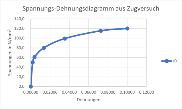
Relating the force to the initial cross-section of the specimen and the displacement to the length of the specimen results in the so-called engineering stress-strain diagram (see Figure 1).
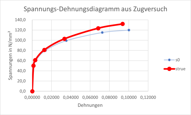
However, since the cross-section of the specimen changes due to necking, it is possible to determine the so-called "true stresses and strains" under the assumption that the volume remains the same, which are usually used as material data in a finite element analysis FEM.
Since the true stresses are always greater than the technical ones, one can also apply the technical values for the sake of simplicity (a few steps to the safe side of the abyss to the right).
Example
Let's make a simple example:
For an aluminum material we find the specifications:
Yield strength Rp0.2 = 50 N/mm²
Tensile strength Rm = 120 N/mm²
Elongation at break A5 = 10
E-modulus E = 70,000 N/mm²
Here we are dealing with the technical characteristic values.
With these values, we at Merkle CAE Solutions can already roughly describe the plastic material behavior if the more precise values of the tensile test (see Figure 2) are not available.
A conversion to the true stresses and strains gives:
Yield strength Rp0.2 = 50.1 N/mm²
Tensile strength Rm = 132 N/mm²
Elongation at break A5 = 9.12
E-modulus E = 70,000 N/mm²
Here it can be seen that the yield strength and tensile strength increase somewhat, while the elongation at break decreases somewhat. At smaller strains, however, the curves are almost congruent.
The plastic behavior can also be characterized by two straight lines. This is called a bilinear material model. This has the charm that the values for this can be taken directly from a table book (Figure 3).
If you don't want to bother with the calculations and would rather go one step further to the right, you can use the technical values (blue curve) for the calculation instead of the true values (red curve). This will result in higher and higher elongations at a certain stress.
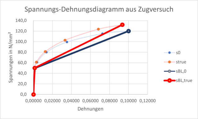
But it's even simpler than that: the elastic strains at yield strength Rp0.2 (0.2% plastic strain = 0.002) are much smaller in low cycle fatigue than the actual plastic strains, which are in the range of perhaps 1-5%.
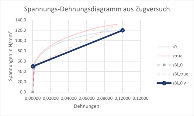
The curve is not visibly different from the bilinear law and is very simple: the point of intersection with the y-axis is the yield strength and the second point is the tensile strength at elongation at break (see Figure 4).
Life Cycle
But now to the service life (how many steps can I take towards the abyss). In the LCF, incremental plastic strain plays an essential role.
We now assume that during a load change the material is locally stressed beyond the yield point, e.g. a radiator heats up and cools down again (1 load change).
Plastic strains occur at the critical point once as tension and once as compression. Tension is usually more critical than compression, since microcracks propagate under tensile stresses, while cracks close under compression.
To be on the safe side, tension and compression are evaluated equally in a finite element calculation and the plastic strains occurring per load change (incremental plastic strain) are simply added up in terms of amounts.
The technical term for this is cumulative plastic strain.
In order to determine the service life, i.e. the maximum load cycles that can be tolerated, we check how often the incremental plastic strain can be added to the cumulative plastic strain until it reaches the ultimate strain.
Using a finite element calculation, we at Merkle CAE Solutions can calculate several load cycles on a component and estimate the course of the sum of the incremental plastic strains using a suitable function. If the difference increases from cycle to cycle, the function is an e-function; if it remains constant, the result is a linear function; if it decreases, the result is a logarithmic function.
For systems subject to high thermal loads, such as exhaust systems and coolers, you will find that logarithmic functions usually result. If the expected function type is known, one calculated cycle is sufficient to estimate the number of load cycles that can be tolerated.
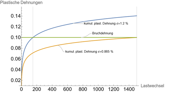
Figure 5 shows the load cycles that can be tolerated at two plastic strains. Let us assume that we have calculated a tolerable number of load cycles of 150 load cycles (e=1.2%) in the model with the material parameters assumed above. However, the test showed that failure only occurred at 1,500 load cycles (e=0.865%).
The question now arises as to how much higher the yield strength of the material would have to be for the test and the calculation to agree.
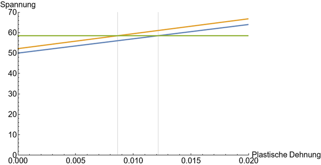
The simplified material model in Figure 6 gives us the answer:
To get from a plastic strain of about 1.2% to 0.865%, it is mathematically sufficient to increase the yield strength in the material model from 50 N/mm² to 52 N/mm².
Since material properties are usually minimum values with a scatter range of several percent, this alone can explain the difference in service life. Another effect that leads to a higher yield strength is the cyclic hardening of a material, which is usually neglected for lack of corresponding data.
A higher yield strength alone, in this case of 4% from 50 to 52 N/mm², is sufficient to explain the discrepancy of 150 load cycles to 1,500 load cycles. The measured yield strength of a batch is often far more than 4% above the specified minimum yield strength.
Conclusion
It can also be expressed as follows: a calculated factor of 10 for the actual service life to the calculated one is a really good calculation result in the LCF range if we are on the right side of the edge, i.e. if the calculated service life is smaller than the one observed in the test.
When reconciling calculation and test, the material law can be adjusted as long as the changes are physically plausible.
Since this topic is often not completely clear to many customers of Merkle CAE Solutions, I have clarified it for you here using a concrete example.
Yours Stefan Merkle

PS: The Low Cycle Fatigue test (LCF) according to ISO 12106 and ASTM E606 is a fatigue test in which cyclic loading to failure is simulated. The test is typically performed on a servo-hydraulic testing machine.